Robert Lowe

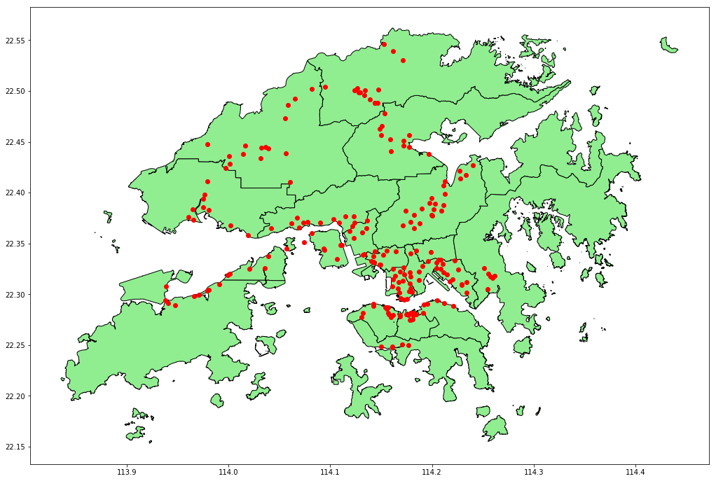
In my previous post I talked about using GeoPandas to visualise geolocation data (the locations of traffic cameras in Hong Kong). In this post I’m going to discuss using the Amazon SageMaker machine learning platform to group these locations using k-means clustering. (Perhaps there is budget for a fixed number of traffic camera maintenance stations, and we want to determine the optimal locations.) Below is a visualisation of the result with 15 clusters (k = 15), with red dots representing traffic camera locations, and blue triangles representing cluster centroids.

The code that performs the clustering and creates the visualisation is in a Jupyter Notebook. The previous post explains how to run a notebook using SageMaker. Note that SageMaker needs to write artifacts for the model it generates to an S3 bucket, so you’ll need to ensure that the notebook instance is using a role that has permission to write to a suitable bucket.

We start by assigning the name of this bucket to a variable.

bucket_name = '[YOUR-BUCKET-NAME]'

Next we install some packages we will need later, and load the location data.

!pip install --upgrade pip --quiet
!pip install geopandas --quiet
!pip install descartes --quiet
!pip install mxnet --quiet

import pandas as pd

cameras = pd.read_csv('Traffic_Camera_Locations_En.csv')

Training the model

We extract the columns we need, and convert to an ndarray of float32s as required by SageMaker.

train_df = cameras[['latitude', 'longitude']]
train_data = train_df.values.astype('float32')

We also need to generate our own unique name for the training job rather than letting SageMaker assign one, so that we can locate the generated model artifacts later.

from datetime import datetime

job_name = 'traffic-cameras-k-means-job-{}'.format(datetime.now().strftime("%Y%m%d%H%M%S"))

We can use the high-level SageMaker Python SDK to create an estimator to train the model. Note that we are specifying that we want 15 clusters (k=15).

from sagemaker import KMeans, get_execution_role

kmeans = KMeans(role=get_execution_role(),
                train_instance_count=1,
                train_instance_type='ml.c4.xlarge',
                output_path='s3://' + bucket_name + '/',
                k=15)

Now we can train the model. The SDK makes this easy, but there’s a lot going on behind the scenes.

• The SDK writes our training data to a SageMaker S3 bucket in Protocol Buffers format.
• SageMaker spins up one or more containers to run the training algorithm.
• The containers read the training data from S3, and use it to create the number of clusters specified.
• SageMaker writes artifacts for the trained model to the location specified by output_path above, using an MXNet serialisation format, then shuts down the containers.

The process takes several minutes.

%%time
kmeans.fit(kmeans.record_set(train_data), job_name=job_name)

Interpreting the model

While the SageMaker Python SDK makes it straightforward to train the model, interpreting the model (i.e. finding the cluster centroids) requires more work.

SageMaker stores the model artifacts in S3 in the location we specify, so the first step is to download the model artifacts to the notebook instance.

import boto3

model_key = job_name + '/output/model.tar.gz'
boto3.resource('s3').Bucket(bucket_name).download_file(model_key, 'model.tar.gz')

Next, we extract and unzip the model artifacts.

import os

os.system('tar -zxvf model.tar.gz')
os.system('unzip model_algo-1')

Then we can use the MXNet libraries to load the model data into a numpy ndarray.

import mxnet as mx

Kmeans_model_params = mx.ndarray.load('model_algo-1')

Next we turn this into a pandas DataFrame with appropriate column names.

cluster_centroids = pd.DataFrame(Kmeans_model_params[0].asnumpy())
cluster_centroids.columns = train_df.columns

Visualising the results

Now we can use GeoPandas to visualise the results, producing the image shown earlier in this post. For more on mapping geolocation data using GeoPandas, see this notebook.

from geopandas import GeoDataFrame, points_from_xy
import matplotlib.pyplot as plt
%matplotlib inline

plt.rcParams['figure.figsize'] = [19, 12]

hong_kong = GeoDataFrame.from_file('Hong_Kong_18_Districts/')
cameras_geo = GeoDataFrame(cameras, geometry=points_from_xy(cameras.longitude, cameras.latitude))
centroids_geo = GeoDataFrame(
    cluster_centroids, geometry=points_from_xy(cluster_centroids.longitude, cluster_centroids.latitude))
axes = hong_kong.plot(color='lightgreen', edgecolor='black')
cameras_geo.plot(ax=axes, color='red')
centroids_geo.plot(ax=axes, marker='^', color='blue', markersize=100)

The complete source code, including the datasets, is available on GitHub.

Conclusion

Does it really make sense to use SageMaker for this problem? Well, no. SageMaker works by spinning up separate containers to perform the training, with both the training data and the resulting model written to S3. That’s a lot of overhead, and takes several minutes even for a very small dataset such as this one. We could perform the same processing in-memory on the notebook instance itself in a fraction of the time using, for example, scikit-learn.

However, by using SageMaker we’re familiarising ourselves with a process that can scale to far larger datasets. In fact, using pipe mode we can stream training data directly from S3, so it’s not even necessary for the dataset to fit on the local volume(s) attached to our training instance(s).

Recently I’ve had cause to work with geospatial data in Amazon SageMaker and needed a way to visualise the results. I’ll write more about SageMaker itself in a future post. In this post I aim to summarise a bit of what I learned about working with geospatial data in Python, in particular using GeoPandas.

I created a Jupyter Notebook that demonstrates how to use GeoPandas to load a set of points, in this case locations of traffic cameras in Hong Kong (as it happens, from the same dataset I used to create this), and layer them on top of a shapefile representing a map of the 18 districts of Hong Kong, resulting in a visualisation such as the one below.

The complete source code is available on GitHub.

Using Amazon SageMaker Notebooks

This code will run in any Jupyter environment. I used an Amazon SageMaker Notebook, as described below. Amazon SageMaker is part of AWS, so you will need an AWS account to follow this approach.

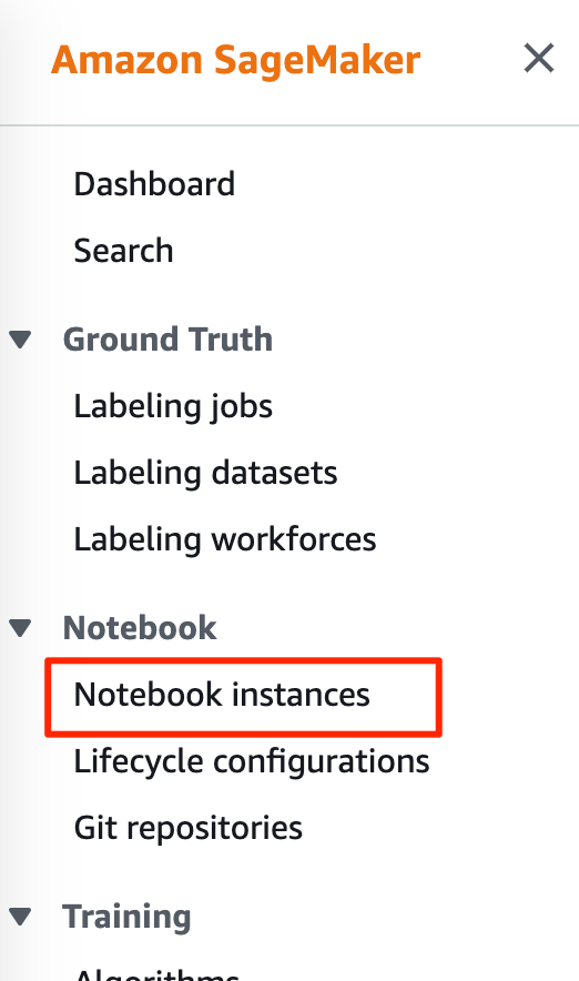
Start by navigating to Amazon SageMaker in the AWS console. In the Amazon SageMaker menu, under Notebook, select Notebook instances.

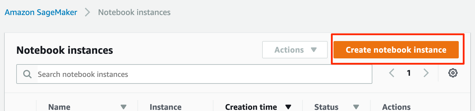
On the Notebook instances page, click Create notebook instance.

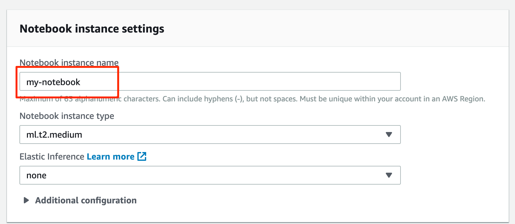
Under Notebook instance settings, give your instance a name.

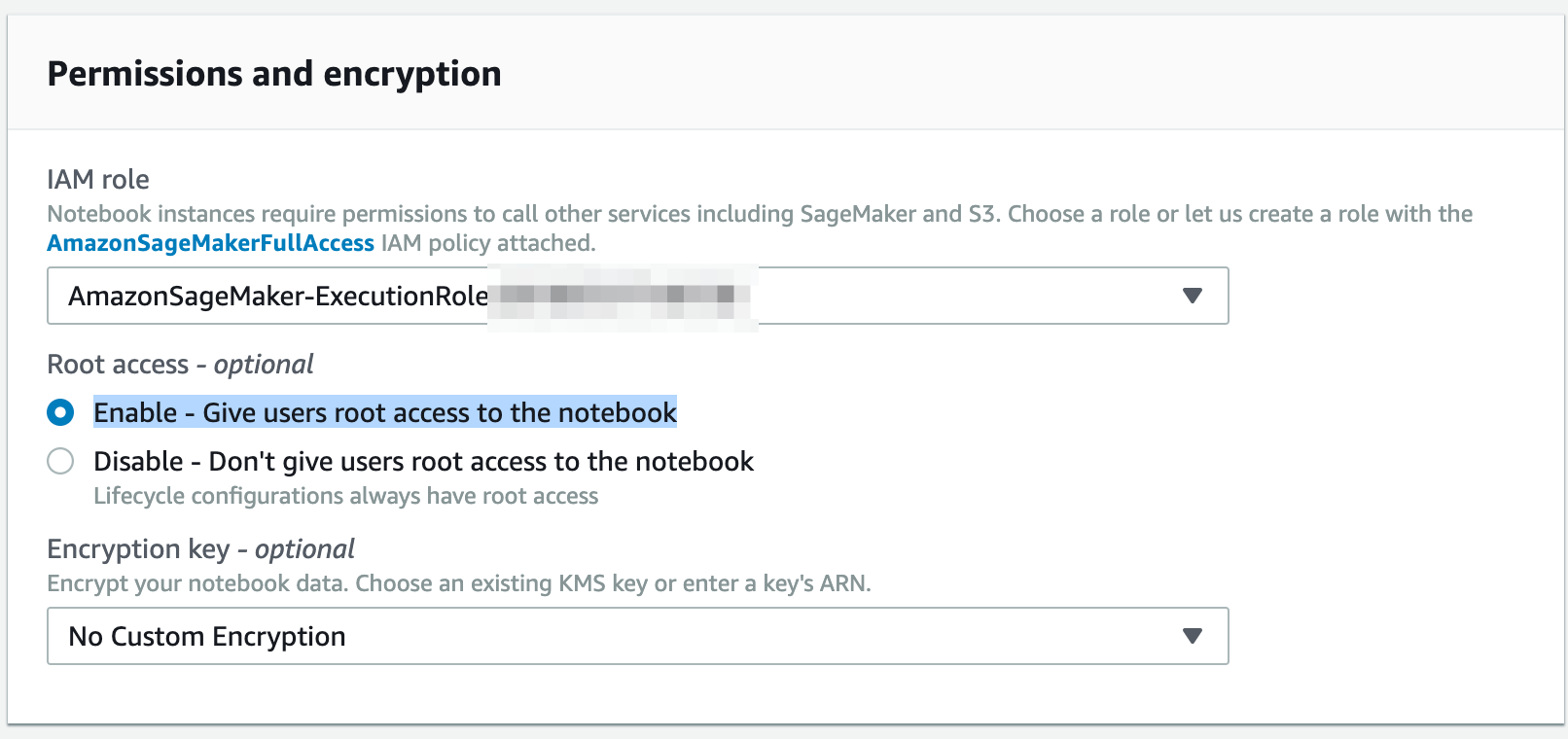
Under Permissions and encryption, if you don’t already have a SageMaker role, choose Create a new role under IAM role. The role defaults should be fine as the notebook doesn’t require any special permissions. Under Root access select Enable – Give users root access to the notebook.

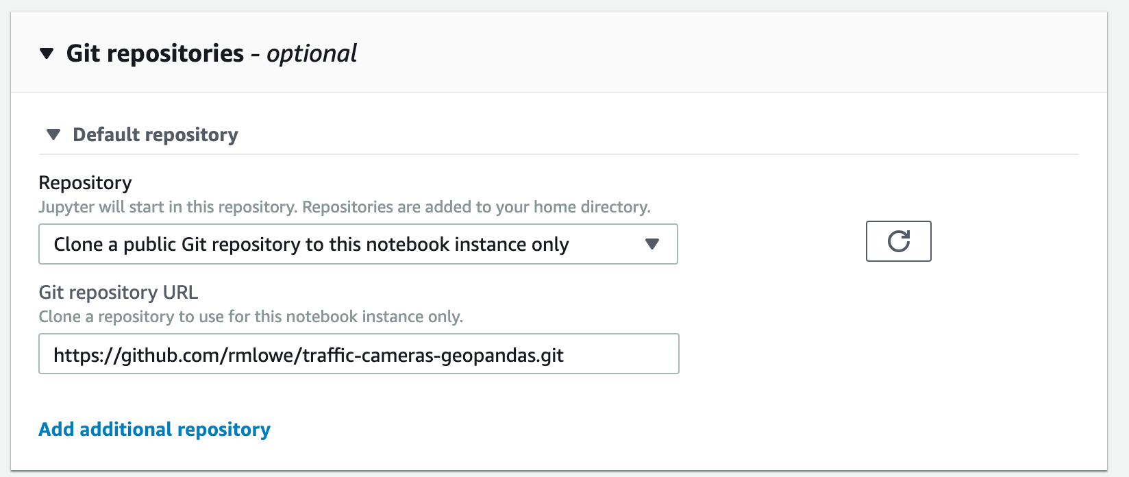
Under Git repositories, choose Clone a public Git repository to this notebook instance only. Under Git repository URL, enter the URL of the repository, which is https://github.com/rmlowe/traffic-cameras-geopandas.git.

Alternatively, you could fork this repository, and then add the forked repository to your Amazon SageMaker account. That allows you to associate credentials with the repository in SageMaker, so you can push changes back up to the forked repository.

You can leave other settings at their default values, and click Create notebook instance.

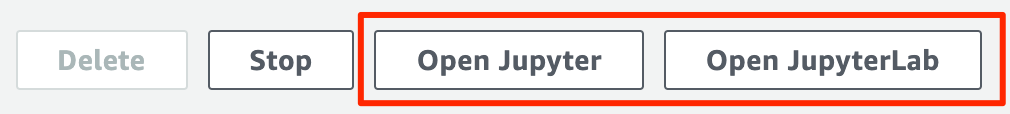
It might take a few minutes for the instance to start. Once the instance is started, click on the instance name under Notebook instances, then click on either Open Jupyter or Open JupyterLab to access the notebook. (I recommend using JupyterLab since it has out-of-the-box integration with git.)